How-to Import Multibeam Bathymetry Into GRASS Using MB-System

This how-to exercise covers the basic steps I use to import multibeam data into GRASS using MB-System. The multibeam data used for this exercise are a portion of the Loihi data available from the MB-System download page.

You should already have GRASS, GDAL, and MB-System installed. Also, you need to download and extract the Loihi data.

For this exercise, you also need to download the Add-On programs mb_nav_ogr and r.in.mb available from this site. These programs simplify the process of moving multibeam data into GRASS for post-processing.

NOTE: This how-to exercise describes how to to import multibeam bathymetry using the GRASS wxPython Graphical User Interface (GUI). In my next post, I describe the same procedures using the GRASS command line interface.

Before you start, you need to setup a GRASS location for UTM Map Zone 4N referenced to WGS84. The EPSG code for this location is 32604. The basic steps to import multibeam data into GRASS using MB-System include:

Creating a data list and extracting navigation.
Importing navigation into GRASS and setting the map region.
Gridding the multibeam bathymetry.
Assigning a color table to the gridded bathymetry.
Creating a sun-illuminated bathymetry map.
Creating a color-shaded bathymetry map.

Step 1: Creating a Data List and Extracting Navigation

For this exercise, you are working with the GSF (MB ID=121) multibeam data in the SumnerLoihi1997 folder of the Loihi dataset.

NOTE: The Loihi dataset contains both raw and processed multibeam data, plus any related ancillary files (fast bathy, fast nav, etc).

To create a new MB-System data list for the SumnerLoihi1997 folder, run this command.

ls SumnerLoihi1997/*.d01 SumnerLoihi1997/*.d02 | awk '{print $1" 121 1.0"}' > SumnerLoihi1997_data_list.txt

This produces a list of the unprocessed multibeam data in the SumnerLoihi1997 folder. You can use a similar command to list the processed data.

ls SumnerLoihi1997/*p.mb121 | awk '{print $1" 121 1.0"}' > SumnerLoihi1997_data_list.txt

Extract the navigation as an ESRI Shapefile using the mb_nav_ogr command.

mb_out_nav -i SumnerLoihi1997_data_list.txt -o sumnerloihi1997_navigation.shp -p EPSG:32604

The extracted navigation file sumnerloihi1997_navigation.shp is now ready to import into GRASS.

Step 2: Importing Navigation Into GRASS and Setting the Map Region

From the GRASS GIS Layer Manager, select File->Import vector data->Common import formats [v.in.ogr].
The Import vector data dialog opens.
Using the Browse button in the Source section, select the Shapefile sumnerloihi1997_navigation.shp. Ensure Add imported layers into layer tree is selected.
To import the Shapefile into GRASS, select Import.
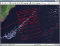
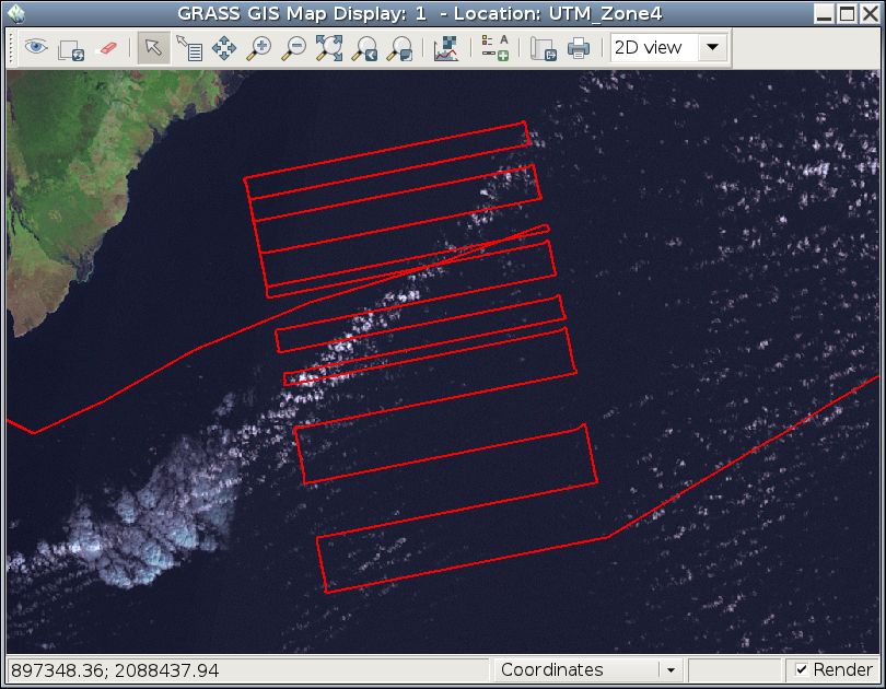
The imported GRASS vector is saved with the same filename minus the ".shp" extension ( sumnerloihi1997_navigation).

At this point, you can change the display properties of the imported navigation. The imported navigation can also be queried based upon import attributes (Name, Year, Julian Day, Distance, Total Time). You can now use the imported navigation to the set the region for gridding the bathymetry. It is also a useful way to inspect the navigation for any any errors. If there are errors in the navigation, edit the problem file(s) with mbnavedit, and repeat the above import process.

From the Map Display, use the Zoom buttons to adjust the GRASS Region.
For this example, I focused on the mosaic block ignoring the transit lines to the east and west.
To apply the current display region from the Map Display, select Various zoom options->Set computational region from display extent.
After the region extent is set, the region resolution must be set. The region resolution determines the resolution of the gridded multibeam map.
To set the GRASS region resolution, select Settings->Region->Set Region [g.region].
The g.region dialog opens.
Under the Bounds tab in the the g.region dialog, select Align region to resolution. Under the Resolution tab, enter a value (50) in the Grid resolution 2D box.
For this example, use a resolution of 50 meters.
To apply the new region resolution, select Run.

The GRASS region has now been set and you are ready to grid the multibeam bathymetry.

Step 3: Gridding the Multibeam Bathymetry

To grid the multibeam bathymetry, use the r.in.mb GRASS add-on.

From the Command console tab in the Layer Manager window, type r.in.mb and press Enter.
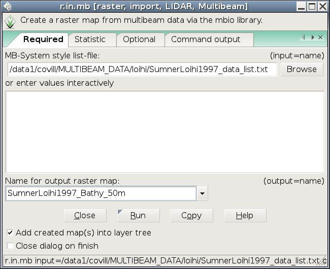
The r.in.mb dialog opens.
Under the Required tab using the Browse button, select the MB-System data list SumnerLoihi1997_data_list.txt.
In the Name for output raster map box, type the name for the new GRASS file.
For this example, create a new GRASS raster called SumnerLoihi1997_Bathy_50m.
To begin the gridding process, select Run.
The importing and gridding process display in the Command output tab of the r.in.mb dialog. The new map displays automatically when the gridding is complete.

NOTE: This example uses the default gridding options for r.in.mb. The dialog provides several options to control the gridding process including:

Gridding method (default = mean).
Restricting by acrosstrack width and beam number.
Restricting by speed and line length.
Restricting by depth range.

Consult the r.in.mb Help page for more information.

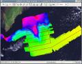To make the NULL (empty) values in the raster transparent, in the Map Layers tab, double-click the SumnerLoihi1997_Bathy_50m raster. In the Null cell tab of the d.rast dialog, select Overlay and OK.

The gridded multibeam bathymetry is now ready for post-processing with the GRASS GIS. At this point, you have several options for post-processing the gridded data including:

Smoothing with r.neighbours.
Visualizing in 3-D with NVIZ.
Generating contours with r.contour.

Step 4: Assigning a Color Table to the Gridded Bathymetry

To assign a color table to the imported bathymetry, in the Layer Manager, select Raster->Manage colors->Color tables [r.color].
The r.colors dialog opens.
From the Name of input raster map menu, select the name of the gridded bathymetry (SumnerLoihi1997_Bathy_50m).

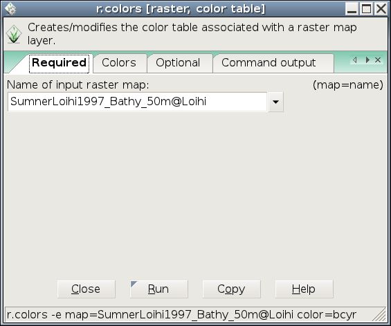
Hint: If the raster is already selected in the Layer Manager, the name is automatically added to the dialog.

From the Type of color table menu in the Colors tab, select a color table.
Use the blue-cyan-yellow-red (bcyr) color table. This assigns red to the shallow depths down through blue for the deepest. The haxby color table also works well.
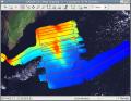
To apply the new color table to the imported bathymetry, select Run.
The imported bathymetry automatically re-draws in the Map Display with the new color table.

By default, the color table is spread evenly over the depth range for the selected raster. To apply the colors based upon data distribution (not depth range), from the Colors tab, select Histogram equalization.

You are now ready to create a sun-illuminated bathymetry map.

Step 5: Creating a Sun-Illuminated Bathymetry Map

You are now ready to create a grey, sun-illuminated map from the imported bathymetry.

To create a sun-illuminated map, in the Layer Manager, select Raster->Terrain analysis->Shaded relief [r.shaded.relief].
The r.shaded.relief dialog opens.
From the Input elevation map menu, select the name of the gridded bathymetry (SumnerLoihi1997_Bathy_50m).
Under the Optional tab in the Output shaded relief map name box, type a name for the sun-illuminated map.
Use SumnerLoihi1997_Bathy_50m_shade.
Under the Optional tab, set the sun altitude, sun azimuth, and vertical exaggeration.
Use a sun altitude of 30 degrees (default), a sun azimuth of 230 degrees, and a vertical exaggeration of 5x.
To create the new sun-illuminated map from the imported bathymetry, select Run.
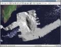
When the shading process is complete, the new sun-illuminated bathymetry map automatically draws in the Map Display.

You are now ready to combine the sun-illuminated map with the color bathymetry.

Step 6: Creating a Color-Shaded Bathymetry Map

You need to combine the color bathymetry with the grey sun-illuminated map to make a color-shaded bathymetry map.

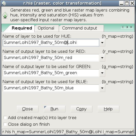
To combine the color bathymetry from Step 4 with the grey sun-illuminated map from Step 5, in the Layer Manager, select Raster->Manage colors->RGB to HIS [r.his].
The r.his dialog opens.
Under the Required tab in the Name of layer to be used for HUE menu, select the name of the color bathyemtry. Type the name for the output red, green, and blue maps (RGB), and unselect Add created map(s) into the layer tree.
Use SumnerLoihi1997_Bathy_50m_red, SumnerLoihi1997_Bathy_50m_green, and SumnerLoihi1997_Bathy_50m_blue respectively.
Under the Optional tab in the Name of layer to be used for INTENSITY menu, select the name of the shaded bathyemtry map. Select Respect NULL values while drawing.
To combine the color bathymetry (HUE) with the sun-illuminated bathymetry (INTENSITY), select Run.
Output from this process consists of three maps, one for red, green, and blue (RGB).
To create the final map, in the Layer Manager, select Raster->Manage colors->Create RGB [r.composite].
The r.composite dialog opens.
Under the Required tab, select the previously created red, green, and blue maps (SumnerLoihi1997_Bathy_50m_red, SumnerLoihi1997_Bathy_50m_green, and SumnerLoihi1997_Bathy_50m_blue).
In the Name for output raster map box, type a name for the output combined map.
Use SumnerLoihi1997_Bathy_50m_combined for output map.
To create the color sun-illuminated map, select Run.
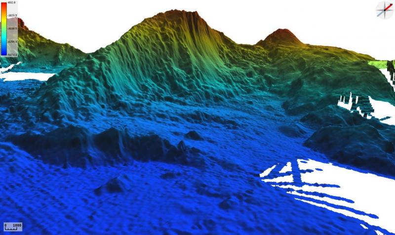
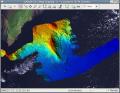
When the process finishes, the new color sun-illuminated bathymetry map automatically draws in the Map Display.